In our discussion on creating a C3 chart a few weeks ago, we generated a great deal of discussion. The concept of cohort analysis obviously hit home and quite a few of you wanted to know more. Specifically, we received numerous requests for guidance on preparing data for this type of analysis.
In today’s post, we will dive into the specifics of how to properly prepare your data for a successful C3 chart, as well as a broader cohort analysis. All that is required is two pieces of data — unique customer ID and transaction date — to create two important measures — purchase period and acquisition cohort. Let’s dive into the process of turning transaction logs into actionable cohort-level insights.
Why Cohort Analysis Matters
Before we get to the data, let’s remind ourselves why cohort analysis matters in the first place. With the approach to analysis, you can dive deep into the behaviors and patterns of specific groups of customers over a period of time. Unlike traditional segmentation methods based on unchanging characteristics like age or location, cohorts provide dynamic insights based on actual purchase actions. By grouping customers by when they first made a purchase, you can uncover the factors that impact their loyalty and behaviors.
Some important questions that cohort analysis can answer include:
- Customer Retention: How long do customers continue to make purchases after their first transaction?
- Retention Trends: Are newer customers more or less likely to remain loyal over time compared to older cohorts?
- Marketing Effectiveness: Which marketing campaigns bring in the most loyal customers?
Answering these questions can guide your decisions, enhance customer loyalty, refine marketing tactics, and boost profits.
Preparing Your Data
To begin analyzing customer cohorts, you only need two pieces of data: (1) unique customer ID and (2) transaction date. These data will typically come from a transaction log or whatever datasource is used to track who made a purchase (or renewed a service in the case of subscription businesses) and when that purchase was made. Additional data such as sales revenue or profit can add more context to your analysis, but they aren’t necessary for the core cohort analysis.
The first step is to group transaction dates into weekly, monthly, and quarterly intervals. By doing this, we create the time periods that form the basis for our analysis and allow us to examine customer actions at different levels of detail.
When we do this in spreadsheets we use a set of basic functions to transform the date into the period. But we must also think of how we format that period, so the formulas we use become a combination of the basic function wrapped in a second function — the TEXT function. This allows for single-digit weeks and months to be displayed with a leading zero, which is necessary for precise sorting and analysis of data.
Here is the most elegant way I know to convert transaction dates into weekly, monthly, and quarterly intervals:
Step 1: Aggregating Transaction Dates
Starting with a spreadsheet that has the Customer ID and Transaction Date columns, type these formulas into columns to the right of the Transaction Date:
- Weekly Cohorts: Use the formula =TEXT(YEAR([Transaction Date Cell]) & “-” & TEXT(WEEKNUM([Transaction Date Cell]), “00”), “YYYY-MM”) to extract the year and week number from the transaction date. The TEXT function formats the week number (01 – 52 or 53 depending on what day of the week the year begins) with a leading zero for accurate sorting.
- Monthly Cohorts: Use the formula =TEXT(YEAR([Transaction Date Cell]) & “-” & TEXT(MONTH([Transaction Date Cell]), “00”), “YYYY-MM”) to extract the year and month (01 – 12). The TEXT function ensures single-digit months are formatted with a leading zero.
- Quarterly Cohorts: Use the formula =YEAR([Transaction Date Cell]) & “-Q” & CEILING(MONTH([Transaction Date Cell])/3) to extract the year and calculate the quarter (Q1 – Q4).
By aggregating transaction dates, you can capture the majority of purchase cycles, making the analysis relevant to both fast-moving and slower-paced categories.
Step 2: Identifying the Acquisition Date
With a few clicks in Excel or Google Sheets, you can easily pinpoint the exact date of each customer’s first purchase. There are a number of ways to do this, some involving creating a new table that isolates each unique Customer ID, some involving a sophisticated string of formulas nested inside one another.
But for me, the most effective method to finding a customer’s Acquisition Date from a list of purchases is using the MINIFS function. This function allows you to quickly find the earliest transaction date for every individual customer in the most straightforward manner I know.
Add another column to your spreadsheet called “Acquisition Date” and type in this formula:
- Acquisition Date: Use the formula =MINIFS([Transaction Date Column], [Customer ID Column], [Customer ID Cell]) to find the first transaction date for each customer based on their unique ID.
Pesto! You’ll now have each unique customer’s Acquisition Date recorded on each line of your spreadsheet. Even when a customer makes a repeat purchase, that Acquisition Date will always be the same.
(It’s not a bad idea to check that in your spreadsheet by sorting it by Customer ID and making sure that the Acquisitions Dates for each customer are consistent. If they’re not, take a close look at your formulas).
Step 3: Creating Acquisition Cohorts
Once you have the Acquisition Dates in hand, apply the same formulas we used to transform the Transaction Date to weekly, monthly, and quarterly periods to the Acquisition Date. The easiest way is to simply copy & paste the Transaction Period formulas into the columns that are to the right of the Acquisition Date. In this way, the newly pasted columns will point back to the Acquisition Date, just as the copied columns pointed to the Transaction Date.
Here’s what the three new Acquisition Period columns will look like:
- Weekly Acquisition Date: =TEXT(YEAR([Acquisition Date Cell]) & “-” & TEXT(WEEKNUM([Acquisition Date Cell]), “00”), “YYYY-MM”)
- Monthly Acquisition Date: =TEXT(YEAR([Acquisition Date Cell]) & “-” & TEXT(MONTH([Acquisition Date Cell]), “00”), “YYYY-MM”)
- Quarterly Acquisition Date: =YEAR([Acquisition Date Cell]) & “-Q” & CEILING(MONTH([Acquisition Date Cell])/3)
These formulas will produce the Acquisition Periods you need to complete the data preparation task. You’re now ready to build your C3 or conduct any variation of cohort analysis you wish.
Step-by-Step Guide and Practice Dataset
Below, you’ll find a link that will take you to a comprehensive guide that will take you through the process we’ve described step-by-step. Within this guide, you’ll have access to a downloadable dataset that you can use to practice these techniques. These resources will give you the opportunity to apply and refine the techniques discussed in this newsletter, making it easier for you to develop your skills.
🔗 Access Your Exclusive Guide and Dataset
Stay Tuned
Don’t forget to check out the video version of this tutorial on our YouTube channel this Friday. Make sure you’re subscribed to the channel stay up-to-date with our newest tutorials and resources.